Part A. Anamorphic Property of the Fourier Transform
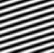
For the first activity, we were first asked asked to create 2D sinusoids in the X direction. The images below are the sinusoids for frequencies of 4, 12 and 20 respectively.


The fourier transforms for the respective sinusoids above are shown below. It can be observed that the greater the frequency value, the farther the white dots are from the center. This is expected. Therefore, it was shown that the frequency of a sinusoid varies proportionally with the distance of the white dot from the image center.


For a constant frequency of 4, the sinusoids were rotated at different theta: 30, 60 and 90 degrees respectively with respect to the vertical axis. The images are shown below.


The resulting FT images show that the dots were also rotated by the same angle. Since the images were in the inverse space, they are directed in the opposite direction. This is as expected of 2D FT images, where rotation of the sinusoids results to the rotation of their FT.


The product of the combination of the 2 sinusoids running in the X and Y directions is shown below with its corresponding FT. The resulting product is like a checkerboard with its alternating white and black square parts, whereas its FT image consists of 4 white dots. Since the dots are located such that it forms like a square, the inversion of the X and Y axes for this FT image is not that evident.


nx = 100; ny = 100;
x = linspace(-1,1,nx);
y = linspace(-1,1,ny);
[X,Y] = ndgrid(x,y);
f = 4 //frequency
z = sin(2*%pi*f*X);nx = 100; ny = 100;
FTz = abs(fft(z));
FFTz = abs(fftshift(FTz));
//imshow(FFTz,[]);
theta = 30;
rotated = sin(2*%pi*f*(Y*sin(theta) + X*cos(theta)));
imshow(rotated,[]);
FTrotated = abs(fft(rotated));
FFTrotated = abs(fftshift(FTrotated));
imshow(FFTrotated,[]);
product = sin(2*%pi*4*X).*sin(2*%pi*4*Y);
//imshow(product,[]);
FTproduct = abs(fft(product));
FFTproduct = abs(fftshift(FTproduct));
imshow(FFTproduct,[]);
Part B. Fingerprints: Ridge Enhancement
For this part of the activity, we were asked to obtain an FT image of a grayscaled fingerprint image, and to determine where the frequencies of the fingerprint ridges are located. This is to enhance the original image by filtering.
The figures below are: the original image, the mean-centered image, its FT image,the filter and the enhanced images.


Here, a high pass filter, was used here to increase the components of the high-frequency and separate it from low-frequency components. This would therefore result in the enhancement of the fingerprint ridges.
It can be observed that fingerprint ridges was enhanced in the output image using the high-pass filter. But, the result was not that clear for the upper and lower parts of the image. The filter radius was varied many times, but the resulting images has more or less the same blurr as the one presented above. Therefore, I think that my program works best for the enhancement of images with lesser blotches or defects than my original image.
fprint = gray_imread('fingerprint.bmp');
fprintmean = fprint-mean(fprint);
imshow(fprintmean);
FT2fprint1 = fft2(fprintmean);
product = real((FT2fprint1).*conj(FT2fprint1));
imshow(fftshift(log(product+1)),[]);
filter = mkfftfilter(fprintmean,'exp',5);
imshow(filter);
FT2fprint2 = FT2fprint1.*fftshift(1-filter);
Image = real(fft2(FT2fprint2));
imshow(Image);
Part C: Lunar Landing Scanned Pictures: Line Removal
For this part, filtering in the Frequency domain was to be done to remove the vertical lines from the given image below. This was first done by applying fft to the grayscaled image of the lunar landing. Using a filter formed through mkfftfilter() of Scilab, it can be observed that white lines were produced by the frequency components. Using a band pass filter between 20 and 100, the last image was formed. Although the resulting image is quite blurry, the aim of the activity which is to remove the vertical lines in the image was accomplished. When the range of the bandpass filter was varied, the vertical lines appeared. Therefore, this is the best image I got so far.


a = imread('moon.bmp');
moon = im2gray(a);
moonmean = moon-mean(moon);
imshow(moonmean);
FTmoon = fft2(moonmean);
product = real((FTmoon).*conj(FTmoon));
imshow(fftshift(log(product+1)),[]);
filter1 = mkfftfilter(moonmean,'binary',100);
filter2 = mkfftfilter(moonmean,'binary',20);
f = filter1-filter2;
image = FTmoon.*fftshift(1-f);
image2 = real(fft2(image));
imshow(image2,[]);
rating - 9 because although I think I did fine in this activity, I was not able to simulate much better output images than those figures I have presented.
Acknowledgement: Angel - for helping me with the enhancement of the fingerprint.
No comments:
Post a Comment