Activity 20: Neural Networks

For this last activity, another pattern recognition model is used to group things in to their proper classes. This model is called Neural Networks, and in the processes implements Error Backprojection (EB). The steps of implementing EB are shown below.


Source: Dr. M. Soriano, A-20 Neural Networks

The objects to be used for this activity are fishballs and squidballs. The input training matrix and desired output wold be set up by extracting 3 features (height/width, R and G chromaticity values), defining 2 classes, with 5 training samples and 5 test samples each. Therefore, the training matrix has 5 rows x 3 columns, while the desired output has 5 rows by 2 columns. The desired output was set to 1 for the fishball class, and 0 for the squidball class.

Activity 19: Probabilistic Classification

In this activity, a different method was implemented to classify images into their proper classes using the features used from the previous activity. The objects used are fishballs and squidballs. There are still 4 training sets and 4 test sets for each object. The features used were still the ratio between the height and the width, and each of their R-G-B values.

Objects used:

The method used here is Linear Discrimination Analysis (LDA), wherein a linear transformation of the features (X) and classes (Y) is determined, such that the transformed values on the new axes maximizes the differences between the features of one class from the other.

The set of features are shown below.

To start, the features were first assigned to their classes (x1= fishballs, and x2=squidballs). Then the mean(μ) was calculated for each class i, and was used to calculate the mean corrected data(xi0) given by the equation:

Then, the covariance matrix (C) was determined using the equations:

The probability (p) that the object feature is assigned to a class i is just the total sample of each class divided by the total samples.

With all the calculated values, the LDA formula given by the equation below, where fi is the linear discriminant, μi is the mean of the feature, C is the covariance matrix, xk is the set of features, and pi is the conditional probability, is used. The object will then be assigned to the class where its calculated linear discriminant is highest.

Results show that:

From the table above, it was shown that 100% of the objects were successfully classified to their proper classes. The objects were assigned to the class where their calculated linear discriminant is highest.

rating: 10 bec. proper classification was done..

Activity 18: Pattern Recognition

In this activity, we were asked to perform classification of different images through pattern recognition. This would be done by assembling different objects, which can be classified into 2 to 5 classes. Half of these will serve as training sets, whereas the other half will serve as test sets. These training set are used to distinguish one class from another.

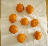
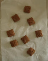
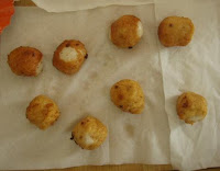
The objects used were fishballs, kwekwek, pillows, and squidballs. I assembled 8 pieces of each of the objects, and classified them using 4 features , which are, the ratio between the height and the width, and each of their R-G-B values.

The objects used are shown below.


The images were first converted into grayscale before the threshold value of the images were determined using their histogram, to be able to properly binarized it.

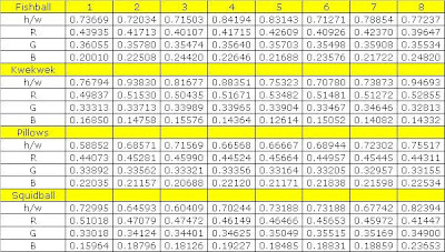
The feature vectors are represented by x, and N is the number of the objects in the each class j.
Below are the feature vectors of the objects.



To determine in which class an unknown feature vector belongs, the feature vector mean given by the equation below is taken.

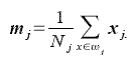
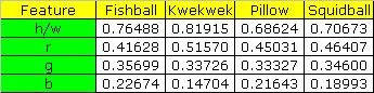
The calculated means are tabulated below.


The calculated mean will then be used to determine the Euclidean distance, D.

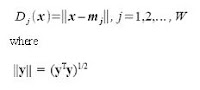
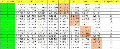
Finally, the class in which minimum Euclidean distance was calculated, is the assigned class of x.
Results from the table below show that 100% of the objects were properly classified.

rating: 10 because proper classification of the objects was done!
acknowledgement: Angel and Marge for helping me with the program.

Activity17: Basic Video Processing

For this activity, we asked to perform an experiment where video processing can be applied to determine the desired kinematic variables. Marge, angel, and I therefore decided to determine the coefficient of restitution of a bouncing object initially dropped at a certain height.

The Coefficient of Restitution for an object that bounces off a stationary object is given by the equation below, where h is the bounce height, and H is the drop height.

C = sqrt (h/H)

To start, the grayscale images of the desired frames acquired from the video using VirtualDub are shown below.

Figures: drop image and bounce image respectively

Due to the inconsistency in the background color and error at the direction at which the video was taken, which were not considered while filming the video, a manual technique was used to determine the coefficient of restitution.

The required heights were measured using Paint. The calculated drop and bounce heights are 60.54 and 54.71 pixels respectively. Therefore, the coefficient of restitution was determined to be 0.95.

rating: 5 bec. image processing was not used

Activity 16: Color Image Segmentation

For this activity, we are asked to perform image segmentation to locate a certain region of interest (ROI) in the image based on colors.

To start with the activity, the RGB colors of an image was represented as normalized chromaticity coordinates (NCC), by dividing each color (R,G,B) with I, as shown by the equations below. Note that it is enough to represent chromaticity by 2 coordinates, ie. r and g.


Segmentation can be done using two methods: probability distribution estimation and histogram backprojection.

In Probability Distribution Estimation, part of the region of interest is cropped and its probability distribution function was determined. The probability that a pixel with chromaticity r, p(r), belongs to the ROI is expressed in the equation below. The mean and the standard deviation are calculated from the cropped part of the region of interest. From the chromaticity coordinates r and g, the joint probability p(r) p(g) function determines if a pixel is part of the region of interest.



Below is the image used for this activity and the cropped part of the ROI.

http://images.google.com.ph/images?hl=tl&q=pink%20objects&um=1&ie=UTF-8&sa=N&tab=wi

The gaussian PDF is:

The resulting segmented image is shown below. It can be observed that the part of the mug where the patch was cropped appears white whereas the other parts appear black. Since the mug was of different shades of pink, the resulting image was not able to reconstruct the whole image of the mug.

For histogram backprojection, a pixel location is given a value equal to its histogram value in
chromaticity space. The figure below shows the superimposed histogram of the cropped portion of the ROI to the chromaticity coordinates, and the resulting image after the backprojection respectively.

Comparing the resulting segmented images using the two methods, it can be observed that the results for the probability distribution function method is much better than that for the histogram backprojection method.

Another image applied with the two methods is shown below, with the results for PDF method and HB method respectively. The first method shows a very good resulting image, whereas the second method has a very faint resulting image.


rating-10, bec the two methods were implemented well. I really enjoyed implementing the methods to different images.

Activity15: Color Camera Processing

For this activity, we are asked to determine the effects of White Balancing (WB) on the quality of captured images.

There are two types of white balancing algorithms, the reference white and the gray world algorithms. In the reference white algorithm, an image is captured using an unbalanced camera and the RGB values of a known white object is used as the divider. On the other hand, for the gray world algorithm, the average red, green and blue value of the captured image are calculated to serve as the balancing constants.

The Red-Green-Blue (RGB) color values for each pixel is given by the equation below,



where:
S(l) = spectral power distribution of the incident light source
r(l) = surface reflectance
n(l) = spectral sensitivity of the camera for red(r), green(g), and blue(b) channels

The following are the images captured using the different WB modes (cloudy, daylight, fluorescent, and tungsten), under the two algorithms of a Canon Powershot a540 digicam.

Figure1. cloudy, reference white algorithm, gray world algorithm

Using the cloudy mode, the image appears warmer than the daylight image below. Implementing the reference white algoritm makes the image appear whiter but less brighter. Using the gray world algorithm, the image becomes darker than the reference white image.

Figure2. daylight, reference white algorithm, gray world algorithm

For the daylight mode, the color of the image seems to remain normal or almost the same as the color seen by the naked eye. Applying the reference white algorithm also makes the image appear whiter but less brighter. Again, the gray world algorithm makes the image darker than the reference white image.

Figure3. fluorescent, reference white algorithm, gray world algorithm

For the fluorescent mode, the image appears brighter than the previous modes. The reference white lessens the brightness and makes the image whiter, while the gray world appears darker.

Figure4. tungsten, reference white algorithm, gray world algorithm

The tungsten mode creates a bluish appearance of the image. After implementing the reference white algorithm, the the image appears darker, but cool colored images. The gray world image again, appears darker than the reference image.

For objects of different shades of blue, applying the 2 WB algorithms results to the images below. The reference white produced an image a little degree whiter than the original image, whereas the gray world produced a brownish colored image. Therefore, reference white is the better algorithm for blue objects in this case.

Figure5. blue, reference white algorithm, gray world algorithm


From the figures, the implementation of the reference white algorithm for each mode produces better quality of images than gray world algorithm. Whereas, the incandescent mode is the worst mode to use considering the nearness of the image colors to the object colors as perceived by the naked eye.

rating-10, because the results of the implementation of algorithms were done successfully!

Activity 14: Stereometry

For this activity, we are asked to reconstruct a 3D image of an object using stereometry, wherein the dimensions (such as depth) of the image are determined.

From the object point (x,y,z), an image is reduced to (x,y) with z projected as a function of x and y and the camera object geometry. By preserving the depth of the image, the 3D image can be inspected at different viewing angles.

In the figure below, considering 2 identical cameras positioned such that the lens centers are at a traverse distance b apart, the image planes of each camera are at a distance f from the camera lens. For an object at point P lying at an axial distance z, P appears in the image plane at a traverse distance x1 and x2 from the centers of the left and right cameras respectively.

To determine the internal parameter f, calibration was done to determine the components of matrix A. Using RQ factorization on A(1:3,1:3), the matrix was converted to a diagonal matrix K given by the expression below,

Then, the x,y coordinates of corresponding vertices in the two images were determined. Using the equation below, z was calculated, and the 3D image of the object was reconstructed.