Activity15: Color Camera Processing

For this activity, we are asked to determine the effects of White Balancing (WB) on the quality of captured images.

There are two types of white balancing algorithms, the reference white and the gray world algorithms. In the reference white algorithm, an image is captured using an unbalanced camera and the RGB values of a known white object is used as the divider. On the other hand, for the gray world algorithm, the average red, green and blue value of the captured image are calculated to serve as the balancing constants.

The Red-Green-Blue (RGB) color values for each pixel is given by the equation below,



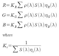
where:
S(l) = spectral power distribution of the incident light source
r(l) = surface reflectance
n(l) = spectral sensitivity of the camera for red(r), green(g), and blue(b) channels

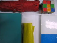
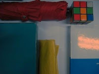
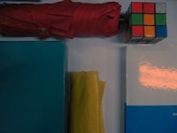
The following are the images captured using the different WB modes (cloudy, daylight, fluorescent, and tungsten), under the two algorithms of a Canon Powershot a540 digicam.

Figure1. cloudy, reference white algorithm, gray world algorithm

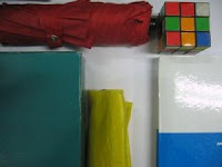
Using the cloudy mode, the image appears warmer than the daylight image below. Implementing the reference white algoritm makes the image appear whiter but less brighter. Using the gray world algorithm, the image becomes darker than the reference white image.

Figure2. daylight, reference white algorithm, gray world algorithm

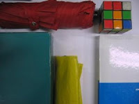
For the daylight mode, the color of the image seems to remain normal or almost the same as the color seen by the naked eye. Applying the reference white algorithm also makes the image appear whiter but less brighter. Again, the gray world algorithm makes the image darker than the reference white image.

Figure3. fluorescent, reference white algorithm, gray world algorithm

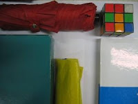
For the fluorescent mode, the image appears brighter than the previous modes. The reference white lessens the brightness and makes the image whiter, while the gray world appears darker.

Figure4. tungsten, reference white algorithm, gray world algorithm

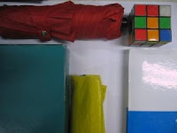
The tungsten mode creates a bluish appearance of the image. After implementing the reference white algorithm, the the image appears darker, but cool colored images. The gray world image again, appears darker than the reference image.

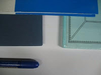
For objects of different shades of blue, applying the 2 WB algorithms results to the images below. The reference white produced an image a little degree whiter than the original image, whereas the gray world produced a brownish colored image. Therefore, reference white is the better algorithm for blue objects in this case.

Figure5. blue, reference white algorithm, gray world algorithm


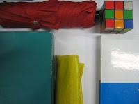
From the figures, the implementation of the reference white algorithm for each mode produces better quality of images than gray world algorithm. Whereas, the incandescent mode is the worst mode to use considering the nearness of the image colors to the object colors as perceived by the naked eye.

rating-10, because the results of the implementation of algorithms were done successfully!

Activity 14: Stereometry

For this activity, we are asked to reconstruct a 3D image of an object using stereometry, wherein the dimensions (such as depth) of the image are determined.

From the object point (x,y,z), an image is reduced to (x,y) with z projected as a function of x and y and the camera object geometry. By preserving the depth of the image, the 3D image can be inspected at different viewing angles.

In the figure below, considering 2 identical cameras positioned such that the lens centers are at a traverse distance b apart, the image planes of each camera are at a distance f from the camera lens. For an object at point P lying at an axial distance z, P appears in the image plane at a traverse distance x1 and x2 from the centers of the left and right cameras respectively.

To determine the internal parameter f, calibration was done to determine the components of matrix A. Using RQ factorization on A(1:3,1:3), the matrix was converted to a diagonal matrix K given by the expression below,

Then, the x,y coordinates of corresponding vertices in the two images were determined. Using the equation below, z was calculated, and the 3D image of the object was reconstructed.

Activity 13: Photometric Stereo

In this activity, we are asked to give an estimation of the shape of a surface or its elevation z by capturing multiple images of it at different locations. Using loadmatfile in scilab, the these four images of the synthetic spherical surfaces which are illuminated by a far away point source located at points V1-4 were loaded:

V1 = {0.085832, 0.17365, 0.98106}
V2 = {0.085832, -0.17365, 0.98106}
V3 = {0.17365, 0, 0.98481}
V4 = {0.16318, -0.34202, 0.92542}

A matrix I was created with the source as the rows, and the x,y,z components of the source as the columns. With N=4 as the number of surface images, matrix I was expressed as:

I1(x , y) = V11 g1+V12 g2+V13 g3
I2(x , y) = V21 g1+V22 g2+V23 g3
IN(x , y) = VN1 g1+VN2 g2+VN3 g3
or I = Vg

The surface normals (nx,ny,nz) were computed by photometric stereo using the equations:
g = ((V '*V)^-1)*V'*I ; where V'= transpose of V
n = g/l; where the normal vector n is determined by normalizing g by its length l

These surface normals are related to a function f by :


Therefore since the elevation z= f(x,y), the surface elevation at point(u,v) is given by f(u,v), and can be calculated using the integral:


The resulting 3D plot of the object shape is shown below:

The code used is:

chdir('C:\Documents and Settings\Plasma\My Documents\julie\186\activity13');
loadmatfile('Photos.mat');

V1= [0.085832 0.17365 0.98106];
V2= [0.085832 -0.17365 0.98106];
V3= [0.17365 0 0.98481];
V4= [0.16318 -0.34202 0.92542];
VN = [V1;V2;V3;V4];
I1= I1(: )';
I2= I2(: )';
I3= I3(: )';
I4= I4(: )';

const = 1e-6;
g = inv(VN'*VN)*VN'*I;
l = sqrt((g(1,:).*g(1,:))+(g(2,:).*g(2,:))+(g(3,:).*g(3,:)));
l = l+const;
for i = 1:3
n(i,:) = g(i,:)./l;
end

dfx = -n(1,: )./(nz+const);
dfy = -n(2,: )./(nz+const);
f1 = cumsum(matrix(dfx,128,128),2);
f2 = cumsum(matrix(dfy,128,128),1);
z = int1+int2;
object = plot3d(1:128, 1:128, z);

rating - 10 because the surface normals were computed and the resulting 3D plot was shown Acknowledgement - Jeric for helping me with the some parts of the code.

Activity 12: Correcting Geometric Distortions

For this activity, we were asked to correct geometric aberrations such as distortion in images as the one shown below.

To start, we were given the distorted image above to work on. The coordinate of the ideal straight image is (x, y), whereas the distorted image has (x',y'). A pixel location was mapped to by some transformation function given by the expression:



A rectangle was created from the most undistorted portion of the image, in this case, at the optical axis of the camera. Here, the number of pixels down and across one box was determined. The four vertices of the corresponding rectangle in both the ideal and the distorted images give the values for the eight unknowns (c1 to c8) in the equations, which are only valid within the polygon. Each vertex also has its corresponding and coordinates.

To compute for the coefficients, the following equations were used:

The location of that point in the distorted image is given by:

If the computed distorted location is integer-valued, the grayscale value is computed from the distorted image onto the blank pixel. Otherwise, the interpolated grayscale value can be computed using the following equation:

The resulting image is therefore:

The code used is:

chdir('G:\186\activity12');
image = imread('image.jpg');
image = im2gray(image);
[x,y] = size(image);
ideal = zeros(x,y);

for i = 1:10:x
ideal(i,:) = ones(y);
//imshow(image)
end
for j=1:8:y
ideal(:, j) = ones(x);
end

xi=[99; 183; 183; 99];
yi=[49; 50; 97; 95];
transpose=[99 48 99*48 1; 245 48 245*48 1; 245 95 245*95 1; 99 95 99*95 1];
c14 = inv(transpose)*xi;
c56 = inv(transpose)*yi;

for i = 1:x
for j = 1:y
imagex = c14(1)*i + c14(2)*j + c14(3)*i*j + c14(4);
imagey = c56(1)*i + c56(2)*j + c56(3)*i*j + c56(4);
if imagex >= x
imagex = x;
end
if imagey >= y
imagey = y;
end
newim(i,j) = image(round(imagex),round(imagey));
end
end
//imshow(newim);

Rating – 9 bec. although the distortion was fixed, the image does not look that good.

Acknowledgement – Jeric for helping me with the code.