Activity 3: Image Types and Basic Image Enhancements II

For the second part of the exercise, the scanned image is shown below:
Due to the large size of the figure, it was reduced to 338 x 640.
To determine the area of the bill, it was first converted into grayscale using gimp. Using its histogram from scilab, its threshold was determined to be 0.937. This was used to convert the figure into a binary image using im2bw(Img,0.937). The resulting image was then inverted by subtracting it from 1, thus resulting to the image below.
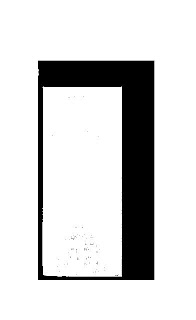
Since there has been a problem with my last activity, I created another program for the determination of the image's area. The resulting area using my program and the converted image is 131323 pixel units2 , which has a %diff. of 1.19% compared with the the actual measured area is 129781 pixel units2. This value is therefore within the allowable 5% difference.

rating-10 because I got a low %difference

Acknowledgements: rica and beth- for helping me with some of the concepts involved
angel - for the conversion of my original image to grayscale

Activity 3: Image Types and Basic Image Enhancements

I. Image Analysis:

The collected images with their corresponding image types are shown below. Using imfinfo('filename') in scilab, their properties were determined.


FileName truecolor.jpg
FileSize 3635
Format JPEG
Width 133
Height 101
Depth 8
StorageType truecolor
No.of Colors 0
XResolution 96
YResolution 96



FileName grayscale.jpg
FileSize 3301
Format JPEG
Width 150
Height 127
Depth 8
StorageType indexed
No.of Colors 256
XResolution 72
YResolution 72


FileName binary.jpg
FileSize 2014
Format JPEG
Width 102
Height 122
Depth 8
StorageType indexed
No.of Colors 2
XResolution 96
YResolution 96

Activity 2: Figure

This is my rectangle figure for the activity.

Activity 2: Area Estimation of Images

The commands I used for the estimation of the area of my rectangle figure are,

a = imread('pic1.bmp');
BWpic1 = im2bw(a, 0 , 1);
[x,y] = follow(BWpic1);
size(x)
size(y)
x1(1) = x(1788);
y1(1) = y(1788);
x2(2:1788) = x(1:1787);
y2(2:1788) = y(1:1787);
A1 = x1(1)*y2(2:1788);
A2 = y1(1)*x2(2:1788);
A3 = A1-A2;
A4 = sum(A3);
Area = 0.5*A4
sum(BWpic1)
area= 196608*0.5

where my x and y sizes are both 1788. The value of the are I got from my program is 98304. But this value has a very high percentage error of 64% compared with the theoretical area which is 59712. The dimension of the rectangle is 311 by 192. I really don't know where the problem lies in my program, since I am quite sure that it is correct. So I'm giving myself a grade of 6 only. Benj, rica, lei and ayeen helped me with some of the problems that I have encountered.

Unfortunately I can't post my figure since I can't upload it now.

Activity 1: Digital Scanning

Figures. Scanned and reconstructed graphs.

From the scanned handwritten graph, coordinates of the given points were determined in Paint. The x and y values of each point were subtracted with the origin's x and y coordinate. The resulting values were then used to reconstruct the graph.

The values used for this activity are tabulated below.

point	x(point)	y(point)	x(final)	y(final)
1	323	689	4	172
2	365	664	46	197
3	408	683	89	178
4	449	609	130	252
5	490	533	171	328
6	532	465	213	396
7	574	459	255	402
8	615	356	296	505
9	655	209	336	652
10	700	411	381	450
11	746	743	427	118
12	786	753	467	108

The grade I'm going to give myself is 9, because I have given enough effort for this activity. Also because the reconstructed graph I got is the same as the scanned graph. Beth, Rica and Benj helped me in clarifying some things.